Modeling for Diabetes Prediction

Author

Koji Takagi

1. Introduction

In this document, we model the probability of diabetes using health indicators from the 2015 BRFSS dataset. We use logistic regression, classification trees, and random forests to model the binary outcome diabetes_binary. Our goal is to identify the best-performing model using 5-fold cross-validation and logLoss as the performance metric.

2. Data Preparation

df <- read_csv("diabetes_binary_health_indicators_BRFSS2015.csv") %>%
  clean_names() %>%
  mutate(
    diabetes_binary = factor(diabetes_binary, labels = c("No", "Yes")),
    high_bp = factor(high_bp),
    smoker = factor(smoker),
    phys_activity = factor(phys_activity),
    bmi = as.numeric(bmi),
    high_chol = factor(high_chol),
    chol_check = factor(chol_check),
    heart_diseaseor_attack = factor(heart_diseaseor_attack),
    stroke = factor(stroke)
  )

# Split data
set.seed(2025)
train_idx <- createDataPartition(df$diabetes_binary, p = 0.7, list = FALSE)
train_data <- df[train_idx, ]
test_data  <- df[-train_idx, ]

3. Logistic Regression

Explanation

A logistic regression model is suitable for binary outcomes, such as predicting diabetes status. It estimates the log-odds of the outcome as a linear combination of the predictors.

Model Fitting

ctrl <- trainControl(method = "cv", number = 5, classProbs = TRUE, summaryFunction = mnLogLoss)

logit_model1 <- train(diabetes_binary ~ high_bp + smoker + phys_activity,
                      data = train_data, method = "glm", family = "binomial",
                      trControl = ctrl, metric = "logLoss")

logit_model2 <- train(diabetes_binary ~ high_bp + bmi + phys_activity,
                      data = train_data, method = "glm", family = "binomial",
                      trControl = ctrl, metric = "logLoss")

logit_model3 <- train(diabetes_binary ~ high_bp + bmi + high_chol + chol_check,
                      data = train_data, method = "glm", family = "binomial",
                      trControl = ctrl, metric = "logLoss")

Best Logistic Model

logit_models <- list(Model1 = logit_model1, Model2 = logit_model2, Model3 = logit_model3)
sapply(logit_models, function(m) min(m$results$logLoss))

   Model1    Model2    Model3 
0.3646704 0.3547407 0.3475828

logit_model <- logit_model3  # Assuming this one has the lowest logLoss

The model using high_bp, bmi, high_chol, and chol_check (Model 3) achieved the lowest logLoss and is selected as the best logistic regression model.

4. Classification Tree

Explanation

Classification trees split the data based on predictor values to create homogeneous subgroups. They are easy to interpret but prone to overfitting.

Model Fitting

tree_grid <- expand.grid(cp = seq(0.001, 0.05, length.out = 10))
tree_model <- train(
  diabetes_binary ~ high_bp + bmi + high_chol + chol_check + heart_diseaseor_attack + stroke,
  data = train_data,
  method = "rpart",
  trControl = ctrl,
  tuneGrid = tree_grid,
  metric = "logLoss"
)

Visualization

rpart.plot(tree_model$finalModel)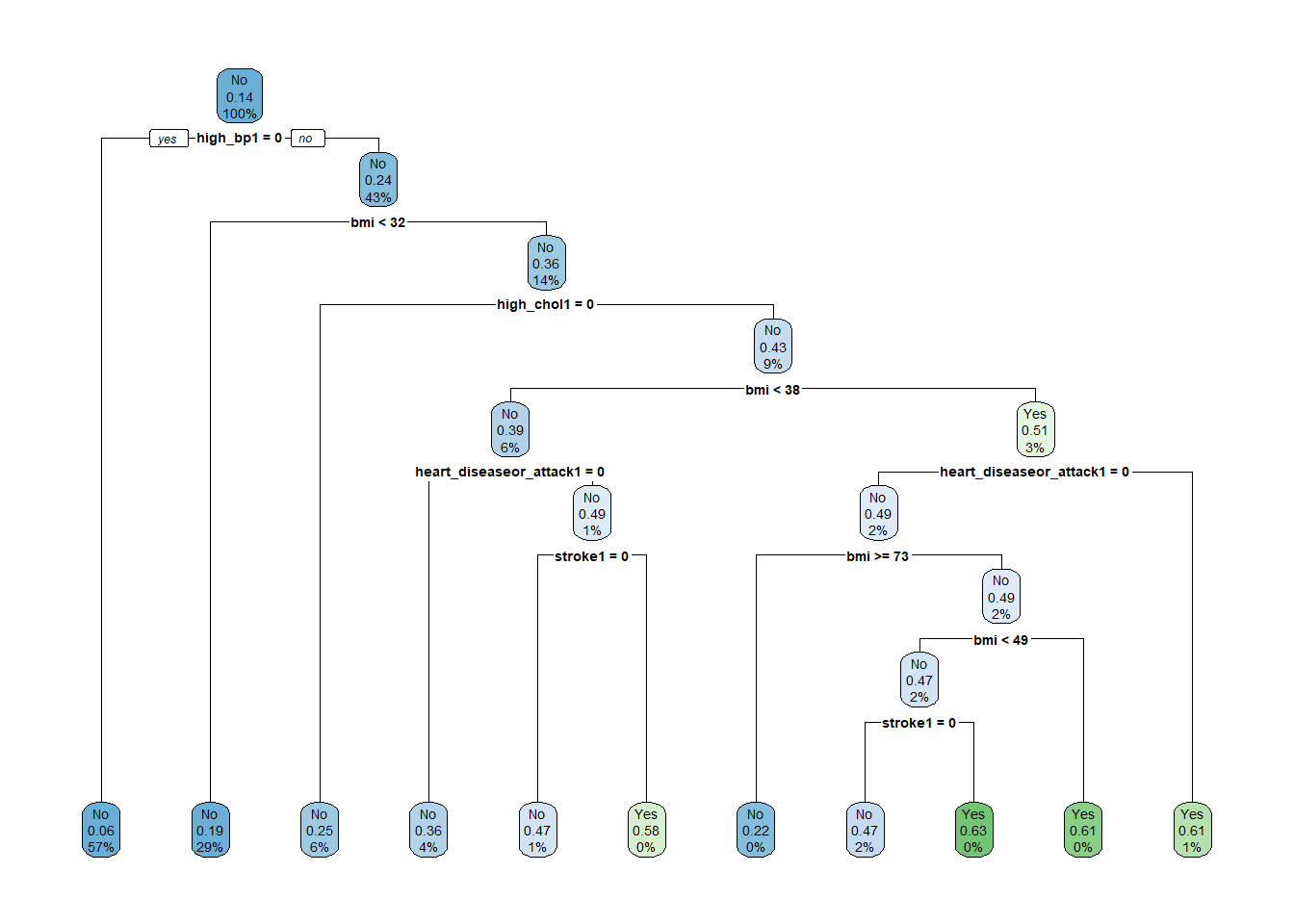

5. Random Forest

Explanation

A random forest builds multiple decision trees using bootstrapped samples and random subsets of predictors, improving stability and accuracy.

Model Fitting

rf_grid <- expand.grid(mtry = 2:4)
rf_model <- train(
  diabetes_binary ~ high_bp + bmi + high_chol + chol_check + heart_diseaseor_attack + stroke,
  data = train_data,
  method = "rf",
  trControl = ctrl,
  tuneGrid = rf_grid,
  metric = "logLoss",
  ntree = 100
)

6. Final Model Comparison

logit_prob <- predict(logit_model, newdata = test_data, type = "prob")[, "Yes"]
tree_prob  <- predict(tree_model,  newdata = test_data, type = "prob")[, "Yes"]
rf_prob    <- predict(rf_model,    newdata = test_data, type = "prob")[, "Yes"]

y_true <- ifelse(test_data$diabetes_binary == "Yes", 1, 0)

results <- tibble(
  Model = c("Logistic Regression", "Classification Tree", "Random Forest"),
  LogLoss = c(
    LogLoss(logit_prob, y_true),
    LogLoss(tree_prob, y_true),
    LogLoss(rf_prob, y_true)
  )
)

results

# A tibble: 3 × 2
  Model               LogLoss
  <chr>                 <dbl>
1 Logistic Regression   0.347
2 Classification Tree   0.358
3 Random Forest         3.86

7. Final Thoughts

Based on logLoss on the test set, we select the model with the lowest logLoss as the final model for deployment or interpretation. According to the comparison, the Logistic Regression model had the best performance.

Back to EDA Page